Introduction to Transmission Matrices

2024-04-01 2633 words 13 minutes

Contents

This blog aims to introduce the concept and use of matrices that characterize two-port networks from a programmatic perspective. First, a theoretical and conceptual review is carried out, and then the development made with code is emulated, working symbolically and vectorially.

Two-port network

Transmission matrices arise from the equations that characterize two-port networks. In general, the matrix that characterizes the transmission of a two-port network can be defined as::

$$ T =\begin{bmatrix} t_{11} & t_{12} \\ t_{21} & t_{22} \end{bmatrix} $$

where each value in the matrix $T$ represents a specific relationship between the input and output of the two-port network.

$$ \begin{align*} t_{11} &= \frac{v_{in}}{v_{out}} \bigg|_{i_{out} = 0} \hspace{8mm} \rightarrow \hspace{8mm} (1 / G_v)\\ t_{12} &= \frac{v_{in}}{i_{out}} \bigg|_{v_{out} = 0} \hspace{8mm} \rightarrow \hspace{8mm} (1 / G_Y)\\ t_{21} &= \frac{i_{in}}{v_{out}} \bigg|_{i_{out} = 0} \hspace{8mm} \rightarrow \hspace{8mm} (1 / G_Z)\\ t_{22} &= \frac{i_{in}}{i_{out}} \bigg|_{v_{out} = 0} \hspace{8mm} \rightarrow \hspace{8mm} (1 / G_i)\\ \end{align*} $$

As can be observed, there are two conditions under which the elements are specified:

$v_{out} = 0$: This indicates that the output voltage is zero, hence the output connectors are short-circuited. $i_{out} = 0$: This implies that the output current is zero, thus the output connectors are open-circuited. This matrix informs us about how to obtain the input variables in terms of the output variables:

$$ \begin{equation*} \begin{bmatrix} v_{in} \\ i_{in} \end{bmatrix} = T \cdot \begin{bmatrix} v_{out} \\ i_{out} \end{bmatrix} = \begin{bmatrix} t_{11} & t_{12} \\ t_{21} & t_{22} \end{bmatrix} \cdot \begin{bmatrix} v_{out} \\ i_{out} \end{bmatrix} = \begin{bmatrix} t_{11} \cdot v_{out} + t_{12} \cdot i_{out}\\ t_{21} \cdot v_{out} + t_{22} \cdot i_{out} \end{bmatrix} \end{equation*} $$

Therefore, to obtain the output variables in terms of the input variables, we must invert the transmission matrix and apply it to the input variables (As long as the determinant of $T$ is different from 0).

$$ T^{-1} = \frac{1}{\det(T)} \cdot \begin{bmatrix} t_{22} & -t_{12} \\ -t_{21} & t_{11} \end{bmatrix} $$

$$ \begin{bmatrix} v_{in} \\ i_{in} \end{bmatrix} = T \cdot \begin{bmatrix} v_{out} \\ i_{out} \end{bmatrix} \hspace{4mm} \rightarrow \hspace{4mm} T^{-1} \cdot \begin{bmatrix} v_{in} \\ i_{in} \end{bmatrix} = \begin{bmatrix} v_{out} \\ i_{out} \end{bmatrix} = \begin{bmatrix} t_{22} \cdot v_{in} - t_{12} \cdot i_{in}\\ -t_{21} \cdot v_{in} + t_{11} \cdot i_{in} \end{bmatrix} \cdot \frac{1}{\det(T)} $$

Moreover, to find the input or output impedance of the system through its respective transmission matrix, a load $Z_L$ is considered at the port opposite to the port being analyzed:

$$ Z_{in} = \frac{t_{11}\cdot Z_L + t_{12}}{t_{21}\cdot Z_L + t_{22}} $$

$$ Z_{out} = \frac{t_{22}\cdot Z_L + t_{12}}{t_{21}\cdot Z_L + t_{11}} $$

With the equations for the output voltage in terms of the input magnitudes and the input impedance, we can derive the formula to calculate the output voltage $v_{out}$ as a function of the input voltage and impedance.

$$ v_{out} = t_{22} \cdot v_{in} - t_{12} \cdot i_{in} = t_{22} \cdot v_{in} - t_{12} \cdot \frac{v_{in}}{Z_{in}} = \Big ( t_{22} - \frac{t_{12}}{Z_{in}} \Big ) v_{in} $$

Transmission matrices

Each component within a circuit has its representation through a two-port network in matrix form. Generally, the matrix representation differs based on whether the components are impedance, admittance, or transformer-based.

Series Impedance transmission matrix ($T_Z$)

$$ T_Z = \begin{bmatrix} 1 & Z \\ 0 & 1 \end{bmatrix} $$

Parallel Admittance transmission matrix ($T_Y$)

$$ T_Y = \begin{bmatrix} 1 & 0 \\ Y & 1 \end{bmatrix} $$

Transformer transmission matrix ($T_T$)

$$ T_T = \begin{bmatrix} n & 0 \\ 0 & 1/n \end{bmatrix} $$

Gyrator transmission matrix ($T_G$)

$$ T_G = \begin{bmatrix} 0 & n \\ 1/n & 0 \end{bmatrix} $$

Finally, the total transfer function of a system is obtained by successively multiplying the transmission matrices of each element. In general, for a system composed of $N$ elements, its transmission matrix will be:

$$ T = \prod_{i=1}^{N} T_i $$

Example 1: Voltage Divider

Let’s consider analyzing the following resistive divider through the transmission matrices of each component to obtain the total transmission of the system.

The idea is to obtain an equation that relates the output quantities (output voltage and output current) in terms of the input quantities (input voltage and input current).

First, we need to define the matrices for both elements. In this case, $R_1$ is in series, but $R_2$ is in parallel, so its transmission matrix should be of the admittance type.

$$ T_{R_1} = \begin{bmatrix} 1 & R_1 \\ 0 & 1 \end{bmatrix} $$

$$ T_{R_2} = \begin{bmatrix} 1 & 0 \\ \frac{1}{R_2} & 1 \end{bmatrix} $$

By performing the successive multiplication of transmission matrices, the total transfer will be:

$$ T = T_{R_1} \cdot T_{R_2} = \begin{bmatrix} 1 & R_1 \\ 0 & 1 \end{bmatrix} \cdot \begin{bmatrix} 1 & 0 \\ \frac{1}{R_2} & 1 \end{bmatrix} = \begin{bmatrix} 1 + \frac{R_1}{R_2} & R_1 \\ \frac{1}{R_2} & 1 \end{bmatrix} $$

Based on the previously described equations, the relationship between the input and output magnitudes becomes:

$$ \begin{equation*} \begin{bmatrix} v_{in} \\ i_{in} \end{bmatrix} = T \cdot \begin{bmatrix} v_{out} \\ i_{out} \end{bmatrix} = \begin{bmatrix} 1 + \frac{R_1}{R_2} & R_1 \\ \frac{1}{R_2} & 1 \end{bmatrix} \cdot \begin{bmatrix} v_{out} \\ i_{out} \end{bmatrix} = \begin{bmatrix} (1 + \frac{R_1}{R_2}) \cdot v_{out} + R_{1} \cdot i_{out}\\ \frac{1}{R_2} \cdot v_{out} + i_{out} \end{bmatrix} \end{equation*} $$

However, in most cases, what we care about is obtaining the output magnitudes as a function of the input magnitudes, so:

$$ T^{-1} = \begin{bmatrix} 1 & -R_1 \\ -\frac{1}{R_2} & 1 + \frac{R_1}{R_2} \end{bmatrix} \cdot \underbrace{\det(T)}_{=1} = \begin{bmatrix} 1 & -R_1 \\ -\frac{1}{R_2} & 1 + \frac{R_1}{R_2} \end{bmatrix} $$

Now we can obtain the output voltage and current as a function of the input voltage and current.

$$ T^{-1} \cdot \begin{bmatrix} v_{in} \\ i_{in} \end{bmatrix} = \begin{bmatrix} 1 & -R_1 \\ -\frac{1}{R_2} & 1 + \frac{R_1}{R_2} \end{bmatrix} \cdot \begin{bmatrix} v_{in} \\ i_{in} \end{bmatrix} = \begin{bmatrix} v_{out} \\ i_{out} \end{bmatrix} = \begin{bmatrix} v_{in} - R_{1} \cdot i_{in}\\ -\frac{1}{R_2} \cdot v_{in} + (1 + \frac{R_1}{R_2}) \cdot i_{in} \end{bmatrix} $$

$$ \begin{align*} v_{out} = v_{in} - R_{1} \cdot i_{in} = v_{in} - v_{R_1} \\ i_{out} = \frac{1}{R_2} \Big ( -v_{in} + R_1 i_{in} + R_2 i_{in}\Big) \end{align*} $$

In Python, all this calculation can be done in several ways. One of them is using symbolic computation with the sympy library.

The symbols to be used are defined and the transmission matrices for the circuit elements are generated.

import sympy as sp

R1, R2 = sp.symbols('R1 R2')

R1_tmatrix = sp.Matrix(
    [[1, R1],
    [0, 1]]
    )

R2_tmatrix = sp.Matrix(
    [[1, 0],
    [1/R2, 1]]
    )

The total transmission is calculated by the successive multiplication of matrices.

# Total transmission matrix
total_tmatrix = R1_tmatrix * R2_tmatrix
display(total_tmatrix)

# Inverse total transmission matrix
inverse_total_tmatrix = total_tmatrix.inv()
display(inverse_total_tmatrix)

# Voltage gain response
voltage_gain_response = sp.simplify((1/total_tmatrix[0,0]))
display(voltage_gain_response)

Multiplying the inverse transmission matrix by the input magnitudes gives:

v_in, i_in = sp.symbols('v_in i_in')
output = inverse_total_tmatrix * sp.Matrix([v_in, i_in])

Example 2: Band-pass filter

The symbols to be used are defined and the transmission matrices for the circuit elements are generated.

import sympy as sp

Z_C1, Z_C2, R1, R2 = sp.symbols('Z_C1 Z_C2 R1 R2')

Z_C1_tmatrix = sp.Matrix(
    [[1, Z_C1],
    [0, 1]]
)

R1_tmatrix = sp.Matrix(
    [[1, 0],
    [1/R1, 1]]
    )

R2_tmatrix = sp.Matrix(
    [[1, R2],
    [0, 1]]
    )

Z_C2_tmatrix = sp.Matrix(
    [[1, 0],
    [1/Z_C2, 1]]
)

The total transmission is calculated by the successive multiplication of matrices. In this case, the magnitude and phase response of the system voltage is sought, so the expression for the voltage gain must be obtained from the transmission matrix.

# Total transmission matrix
total_tmatrix = Z_C1_tmatrix * R1_tmatrix * R2_tmatrix * Z_C2_tmatrix
display(total_tmatrix)

# Inverse total transmission matrix
inverse_total_tmatrix = total_tmatrix.inv()
display(inverse_total_tmatrix)

# Voltage gain response
voltage_gain_response = sp.simplify((1/total_tmatrix[0,0]))
display(voltage_gain_response)

To visualize the response of the system, we must first select values for the components, in this case it is proposed to use:

$$ \begin{align*} R_1 &=& 3.1 ~ k\Omega \\ R_2 &=& 100 ~ k\Omega \\ C_1 &=& 100 ~ nf \\ C_2 &=& 1 ~ nf \\ \end{align*} $$

In turn, a range of frequencies to be represented must be selected, and based on this frequency vector, the impedances must be generated as a function of the frequency for each component.

# Components settings
R1_value = 3_100
R2_value = 100_000
C1_value = 100e-9
C2_value = 1e-9

# Frequency settings
freq_min = 10
freq_max = 10_000
freq_bins = 2048

# Frequency arrays
freq_array = np.logspace(np.log10(freq_min), np.log10(freq_max), num=freq_bins)
angular_freq_array = 2 * np.pi * freq_array

# Impedances as function of frequency
R1_array = np.ones(freq_bins)*R1_value
R2_array = np.ones(freq_bins)*R2_value
Z_C1_array = 1/(1j*C1_value*angular_freq_array) 
Z_C2_array = 1/(1j*C2_value*angular_freq_array)

Finally, the symbolic values of the gain expression must be replaced by the generated impedance vectors.

# Voltage gain array initialization
voltage_gain_array = np.zeros(freq_bins, dtype="complex")

# Loop for replace the symbols by the values of the arrays
for i in range(freq_bins):
    voltage_gain_i = voltage_gain.subs(
        {
            R1: R1_array[i],
            Z_C1: Z_C1_array[i],
            Z_C2: Z_C2_array[i],
            R2: R2_array[i],

        }
    )
    voltage_gain_array[i] = voltage_gain_i

To visualize the response, it is recommended to convert the response of the system magnitude in dB, and to configure the frequency axis in logarithmic scale.

from matplotlib import pyplot as plt

fig, ax1 = plt.subplots(figsize=(10,5))

# Plot for magnitude
ax1.plot(freq_array, 20*np.log10(np.abs(voltage_gain_array)), label="Magnitude", color='b')
ax1.set_xscale('log')
ax1.set_xlabel("Frequency [Hz]")
ax1.set_ylabel("Gain [dB]", color='b')
ax1.set_title("Band-pass response")
ax1.set_ylim(top=0)
ax1.tick_params(axis='y', labelcolor='b')
ax1.grid(True, which="both", ls="--")

# Plot for phase
ax2 = ax1.twinx()
color = 'tab:red'
ax2.plot(freq_array, np.angle(voltage_gain_array)*180/np.pi, label="Phase", color=color)
ax2.set_ylabel("Phase [º]", color=color)
ax2.set_ylim(top=95, bottom=-95)
ax2.tick_params(axis='y', labelcolor=color)
ax2.set_yticks(np.arange(-90, 100, 30))
ax2.set_yticklabels(np.arange(-90, 100, 30))
lines, labels = ax1.get_legend_handles_labels()
lines2, labels2 = ax2.get_legend_handles_labels()
ax1.legend(lines + lines2, labels + labels2, loc='best')

fig.tight_layout()
plt.grid(True, which="both", ls="--")
plt.show()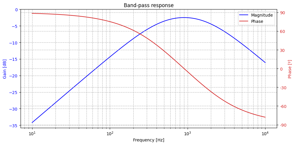

Example 3: RLC filter

So far everything is working great, but there is a not insignificant aspect of all the previous processing that is quite annoying when experimenting with the tool, and that is the execution time and computational cost.

As can be seen in the previous cells, replacing the values frequency by frequency in the symbolic expression takes a long time (30 seconds on average (it’s a lot)).

This is because sympy is a very good tool for working with mathematical expressions, but it is not optimized for vector calculation. Instead, working with libraries like NumPy ensures higher performance since most of its source code is written in low-level languages such as C [1]

For the resonant circuit, we will approach the resolution in a vectorized way with NumPy.

Now, when working in a vectorized way, we won’t be able to initialize a symbolic object and then replace values, but rather the initialization of the matrices must be with the values of the impedances frequency by frequency. Therefore, change the order in which the variables are defined. Now, the first thing we must define is the frequency vector, together with the frequency bins we want to represent.
```
import numpy as np

freq_min = 10
freq_max = 100_000
freq_bins = 2048

freq_array = np.logspace(np.log10(freq_min), np.log10(freq_max), num=freq_bins)
angular_freq_array = 2 * np.pi * freq_array
```
Then, we must decide on the values that the circuit components will have and generate the impedance vectors as a function of frequency for each one. In this case, we adopt the following values:
$$ \begin{align*} R =& 10 ~ \Omega \\ L =& 1 ~ mH \\ C =& 1 ~ \mu f \\ \end{align*} $$
```
R_value = 10
L_value = 1e-3
C_value = 1e-6

R_array = np.ones(freq_bins)*R_value
Z_L_array = 1j*angular_freq_array*L_value
Z_C_array = 1/(1j*angular_freq_array*C_value) 
```

Once the impedances are defined, the transmission matrices of each element are formed. To operate in a vectorized way, the matrices will now have a shape of:

$$ (2\times 2 \times \texttt{freq bins}) $$

Z_L_tmatrix = np.array(
    [[np.ones(freq_bins), Z_L_array],
    [np.zeros(freq_bins), np.ones(freq_bins)]]
)

Z_C_tmatrix = np.array(
    [[np.ones(freq_bins), Z_C_array],
    [np.zeros(freq_bins), np.ones(freq_bins)]]
)

R_tmatrix = np.array(
    [[np.ones(freq_bins), np.zeros(freq_bins)],
    [1/R_array, np.ones(freq_bins)]]
)

print(R_tmatrix.shape)

Up to this point, there isn’t much difference, but now is when the issue gets a bit complicated. When it comes to doing the matrix product, I can no longer use built-in NumPy methods because the multiplication we need to do is not very common. Remembering that matrix multiplication between two matrices can be done if the last dimension of the first matrix is equal to the first dimension of the second matrix, in this case, we’re stuck, because all the transmission matrices will be of $(2\times 2 \times \texttt{freq bins})$.

To solve this problem, we will create a product that we will call “Layer-Wise Dot Product”, since we will be performing the matrix product (Dot product) layer by layer, that is, we will calculate the product for each frequency bin.

def layer_wise_dot_product(*matrices: np.ndarray) -> np.ndarray:
    """
    Performs the sequential layer-wise dot product of multiple 3D matrices along the last dimension.

    Args:
    *matrices: A variable number of 3D numpy arrays.

    Returns:
    A 3D numpy array containing the sequential dot product results for each layer in the last dimension.
    """
    if not all(matrix.shape == matrices[0].shape for matrix in matrices):
        raise ValueError("All matrices must have the same dimensions.")

    result = np.zeros_like(matrices[0])

    _, _, num_layers = matrices[0].shape

    for layer_i in range(num_layers):
        # Start the product with the identity matrix for the first multiplication
        dot_product = np.eye(result.shape[0])
        for matrix in matrices:
            dot_product = np.dot(dot_product, matrix[:, :, layer_i])

        result[:, :, layer_i] = dot_product

    return result

Now we can obtain the transfer function by successively multiplying the transmission matrices. The disadvantage of working in a vectorized way rather than symbolically is that we don’t have the ability to visualize the equations in terms of the components; now we will simply observe a complex matrix.

total_tmatrix = layer_wise_dot_product(Z_C_tmatrix, Z_L_tmatrix, R_tmatrix)

display(total_tmatrix.shape, total_tmatrix)

# Output:
(2, 2, 2048)
array([[[1.  -1591.54314773j, 1.  -1584.22696366j, 1.  -1576.9444109j ,
     ..., 1.    +62.09489201j, 1.    +62.38313291j,
     1.    +62.67269813j],
    [0. -15915.43147734j, 0. -15842.26963657j, 0. -15769.44410902j,
     ..., 0.   +620.94892013j, 0.   +623.8313291j ,
     0.   +626.72698129j]],

   [[0.1    +0.j        , 0.1    +0.j        , 0.1    +0.j        ,
     ..., 0.1    +0.j        , 0.1    +0.j        ,
     0.1    +0.j        ],
    [1.     +0.j        , 1.     +0.j        , 1.     +0.j        ,
     ..., 1.     +0.j        , 1.     +0.j        ,
     1.     +0.j        ]]])

To plot the voltage response in magnitude and phase of the system, we need to obtain the array representing the voltage gain.
```
voltage_gain_array = 1/total_tmatrix[0, 0, :]
```

Similarly to the previous example, it is recommended to convert the system’s magnitude response to dB, and configure the frequency axis in a logarithmic scale.

from matplotlib import pyplot as plt

fig, ax1 = plt.subplots(figsize=(10,5))

# Plot for Gain
ax1.plot(freq_array, 20*np.log10(np.abs(voltage_gain_array)), label="Magnitude", color='b')
ax1.set_xscale('log')
ax1.set_xlabel("Frequency [Hz]")
ax1.set_ylabel("Gain [dB]", color='b')
ax1.set_title("Resonant filter response")
ax1.set_ylim(top=0)
ax1.tick_params(axis='y', labelcolor='b')
ax1.grid(True, which="both", ls="--")

ax2 = ax1.twinx()
color = 'tab:red'

ax2.plot(freq_array, np.angle(voltage_gain_array)*180/np.pi, label="Phase", color=color)
ax2.set_ylabel("Phase [º]", color=color)
ax2.set_ylim(top=95, bottom=-95)
ax2.tick_params(axis='y', labelcolor=color)
ax2.set_yticks(np.arange(-90, 100, 30))
ax2.set_yticklabels(np.arange(-90, 100, 30))
lines, labels = ax1.get_legend_handles_labels()
lines2, labels2 = ax2.get_legend_handles_labels()
ax1.legend(lines + lines2, labels + labels2, loc='best')

fig.tight_layout()
plt.grid(True, which="both", ls="--")
plt.show()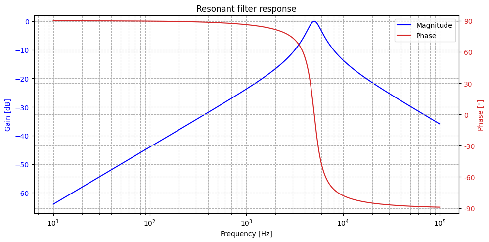

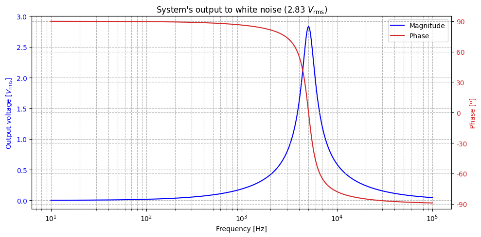
To simulate the signal processing through the circuit, we need to obtain the input impedance. To do this, a load impedance must be established. In this case, we will analyze an open circuit, so:
$$ Z_L = \infty $$
If the load impedance is infinite, then the expression for the input impedance is:
$$ Z_{in} = \frac{t_{11}}{t_{21}} $$
```
# Input impedance
input_impedance = total_tmatrix[0,0,:] / total_tmatrix[1,0,:]
```
With the input impedance defined, we can find the output voltage as a function of the input voltage chosen. In this case, the system is excited with white noise of 2.83 $V_{rms}$.
```
# White noise of 2.83 V RMS
input_voltage = 2.83

output_voltage = (total_tmatrix[1,1,:] - total_tmatrix[0,1,:]/input_impedance) * input_voltage
```

When plotting the output, the unit of measurement is the same as the input unit of measurement ($V_{rms}$).

from matplotlib import pyplot as plt

fig, ax1 = plt.subplots(figsize=(10,5))

# Plot for Gain
ax1.plot(freq_array, np.abs(output_voltage), label="Magnitude", color='b')
ax1.set_xscale('log')
ax1.set_xlabel("Frequency [Hz]")
ax1.set_ylabel(r"Output voltage [$V_{\mathrm{rms}}$]", color='b')
ax1.set_title(r"System's output to white noise ($2.83~V_{\mathrm{rms}}$)")
ax1.tick_params(axis='y', labelcolor='b')
ax1.set_ylim(top=3)
ax1.grid(True, which="both", ls="--")

ax2 = ax1.twinx()
color = 'tab:red'

ax2.plot(freq_array, np.angle(output_voltage)*180/np.pi, label="Phase", color=color)
ax2.set_ylabel("Phase [º]", color=color)
ax2.set_ylim(top=95, bottom=-95)
ax2.tick_params(axis='y', labelcolor=color)
ax2.set_yticks(np.arange(-90, 100, 30))
ax2.set_yticklabels(np.arange(-90, 100, 30))
lines, labels = ax1.get_legend_handles_labels()
lines2, labels2 = ax2.get_legend_handles_labels()
ax1.legend(lines + lines2, labels + labels2, loc='best')

fig.tight_layout()
plt.grid(True, which="both", ls="--")
plt.show()